Basic Information
Local regression or local polynomial regression, also known as moving regression, is a generalization of moving average and polynomial regression. Its most common methods, initially developed for scatterplot smoothing, are LOESS (locally estimated scatterplot smoothing) and LOWESS (locally weighted scatterplot smoothing). From wikipedia
Introduction
- Least Squares finds the line with the minimal squared distance from the data points.
- But how to fit a curve to data?
- LOWESS Smmothing use least squares to do it.
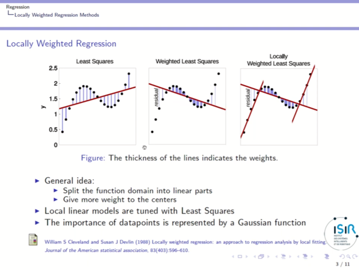
Idea
- Use a type of sliding window to diveide the data into smaller blobs
- At each data point, use a type of least squares(weighted) to fit a line
- To reduce the influence on the new curve, we create an additional weight for the weighted least squares based on how far the original point is from the new point
- Iter
Weight Functions
| Different weight functions | Comparison of weight functions |
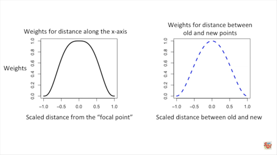 | 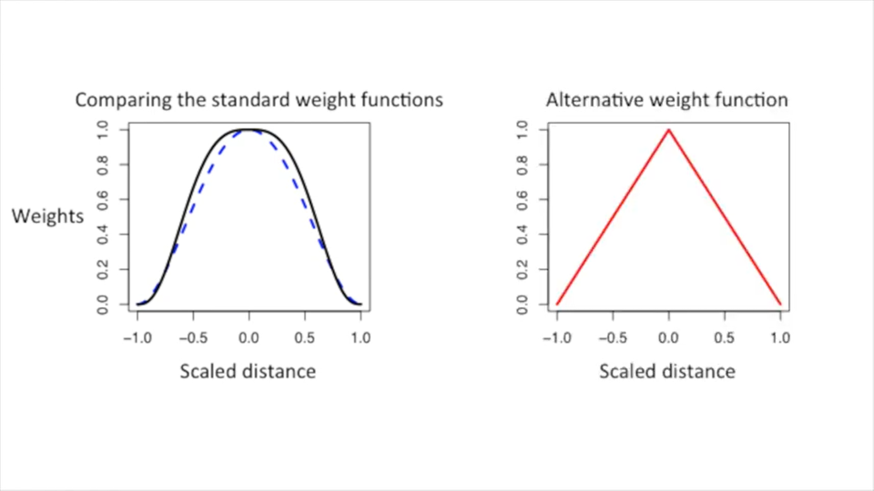 |
Code Example
https://github.com/StatQuest/lowess_loess_demo/blob/master/lowess_loess_demo.R
1
2
3
4
5
6
7
8
9
10
11
12
13
14
15
16
17
18
19
20
21
22
23
24
25
26
27
28
29
30
31
32
33
34
35
36
37
38
39
40
41
42
43
44
45
46
47
48
49
50
51
52
## first let's make a noisy gamma distribution plot...
x <- seq(from=0, to=20, by=0.1)
y.gamma <- dgamma(x, shape=2, scale=2)
y.gamma.scaled <- y.gamma * 100

y.norm <- vector(length=201)
for (i in 1:201) {
  y.norm[i] <- rnorm(n=1, mean=y.gamma.scaled[i], sd=2)
}

data <- data.frame(x, y.norm)

plot(data, frame.plot=FALSE, xlab="", ylab="", col="#d95f0e", lwd=1.5)

## Now that we have the data, let's look at the differences
## and similarities between R's lowess() function and the loess() function.

## We'll start with the lowess() function...
##
## By default "lowess()" fits a line in each window using
## 2/3's of the data points.
##
## the first parameter, y.norm ~ x, says that y.norm is being
## modeled by x, and the second parameter, f, is the fraction
## of points to use in each window. Here, we're using 1/5 of the
## data points in each window.
lo.fit.gamma <- lowess(y.norm ~ x, f=1/5)

plot(data, frame.plot=FALSE, xlab="", ylab="", col="#d95f0e", lwd=1.5)
lines(x, lo.fit.gamma$y, col="black", lwd=3)

## Now use loess() to fit a curve to the data...
##
## By default "loess()" fits a parabola in each window using
## 75% of the data points.
plx<-predict(loess(y.norm ~ x, span=1/5, degree=2, family="symmetric", iterations=4), se=T)

plot(data, frame.plot=FALSE, xlab="", ylab="", col="#d95f0e", lwd=1.5)
lines(x, plx$fit, col="black", lwd=3)

## Now let's add a confidence interval to the loess() fit...
plot(data, type="n", frame.plot=FALSE, xlab="", ylab="", col="#d95f0e", lwd=1.5)
polygon(c(x, rev(x)), c(plx$fit + qt(0.975,plx$df)*plx$se, rev(plx$fit - qt(0.975,plx$df)*plx$se)), col="#99999977")
points(data, col="#d95f0e", lwd=1.5)
lines(x, plx$fit, col="black", lwd=3)

## Now that we know how those functions work... we can skip all that
## nasty stuff and just use ggplot2 with geom_point() and geom_smooth()
library(ggplot2)
ggplot(data=data, aes(x=x, y=y.norm)) +
  geom_point() +
  geom_smooth(span=1/5)