Weighted Gene Co-expression Network Analysis

Standard differential expression analyses seek to identify individual genes

• Each gene is treated as an individual entity
• Often misses the forest for the trees:
  • Fails to recognize that thousands of genes can be organized into relatively few modules

Philosophy of WGCNA

• Unstand the “system” instead of reporting a list of individual parts
  • Describe the functioning of the engine instead of enumerating individual nuts and bolts
• Focus on modules/clusters as opposed to individual genes
  • the greatly alleviates multiple testing problem
• Network terminology is intutive to biologists

Steps

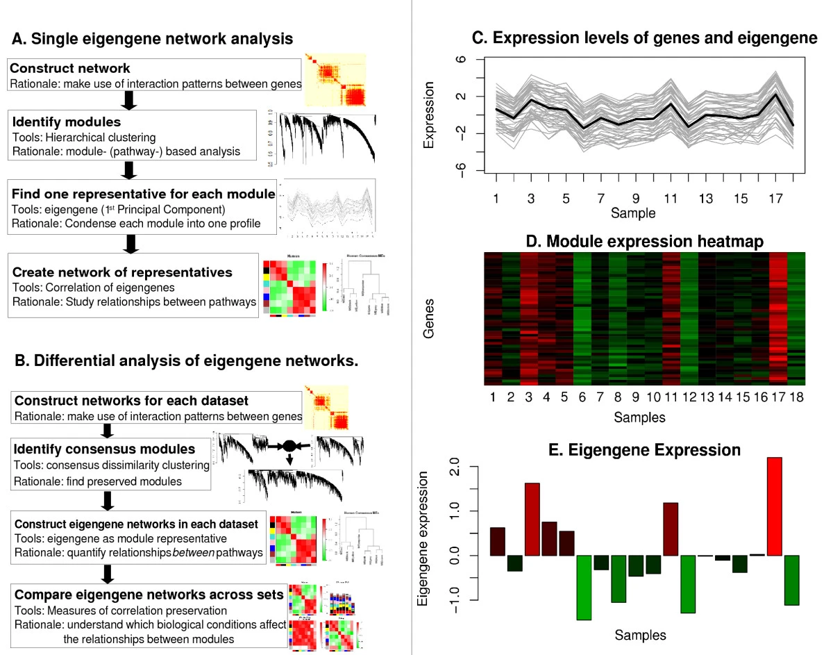
• Construct a network
  • Rationale: make use of interaction patterns between genes
• Identify modules
  • Rationale: module (pathway) based analysis
• Relate modules to external information
  • Array Information: Clinical data, SNPs, proteomics
  • Gene Information: Gene ontology, EASE, IPA
  • Rationale: find biologically interesting modules
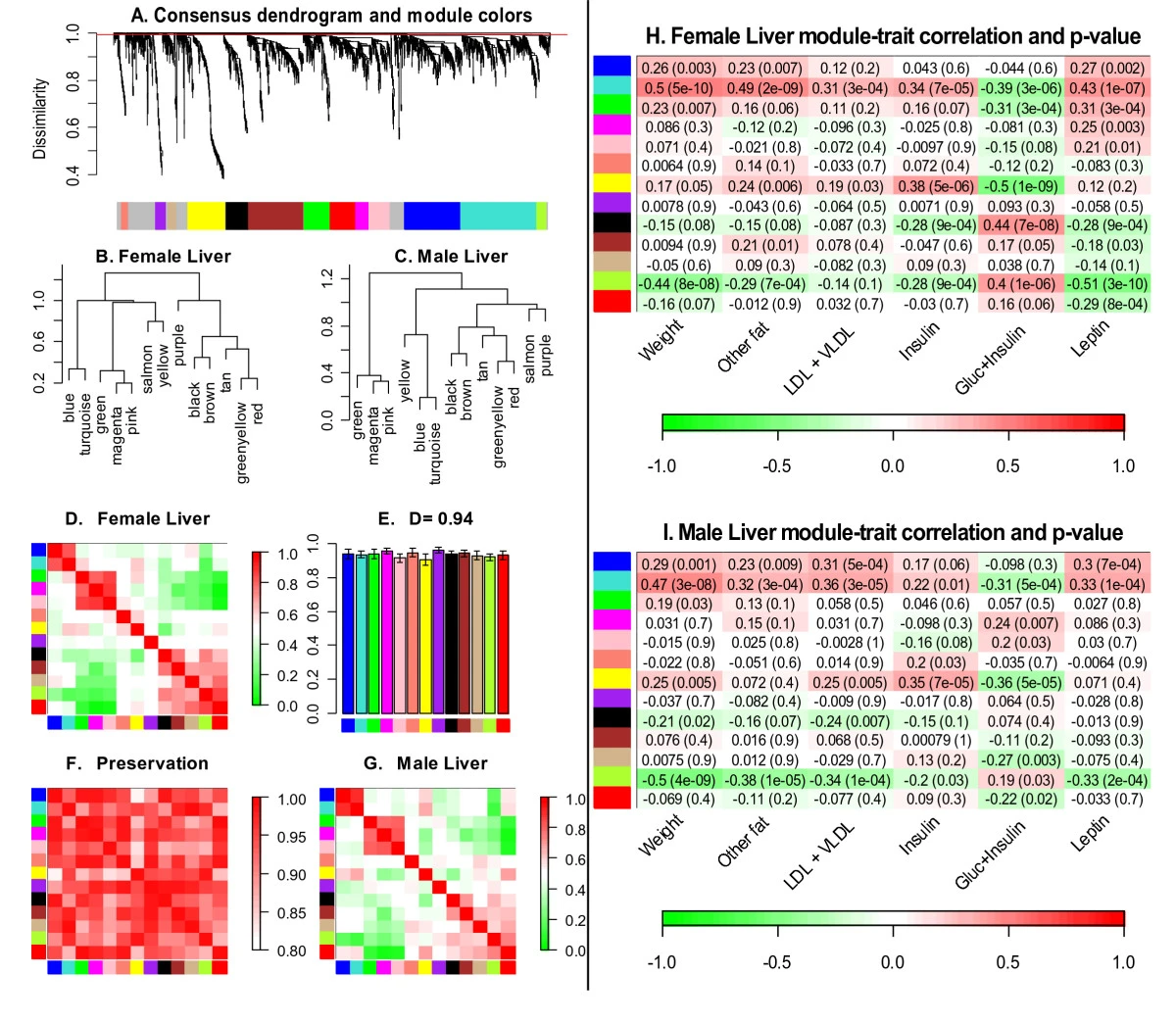
• Study Module Preservation across different data
  • Rationale：
    • Same data: to check robustness of module definition
    • Different data: to find interesting modules
• Find the key drivers in interesting modules
  • Tools: intramodular connectivity, causality testing
  • Rationale: experimental validation, therapeutics, biomarkers

Biologically Meaningful

• reduction of high dimensional data
  • expression: microarray, RNA-seq
  • gene methylation data, fMRI data, etc.
• integration of multiscale data
  • expression data from multiple tissues
  • SNPs (module QTL analysis)
  • Complex phenotype

How to construct

• Network = Adjacency Matrix
• $A=[a_{ij}]$
• A symmetric matrix with entries in [0,1]
• For unweighted netowrk, entries are 1 or 0 depending on whether or not 2 nodes are adjacent (connected)
• For weighted networks, the adjacency matrix reports the connection strength between gene pairs

Steps for constructing a co-expression network

• Gene expression data (array or RNA-seq)
• Measure co-expression with a correlation coefficient
• The correlation matrix is either
  • dichotomized to arrive at an adjacency matrix -> unweighted network
  • OR transformed continuously with the power adjacnecy function -> weighted network

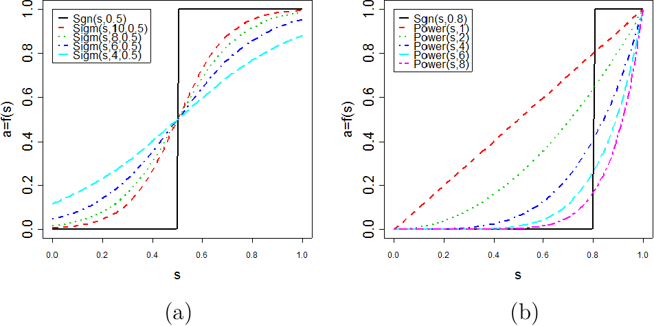
Two types of weighted correlation networks

• Unsigned network, absolute value
  • $a_{ij}=\lvert \text{cor}(x_i,x_j)\rvert^\beta$
• Signed network preserves sign info
  • $a_{ij}=\left\lvert \cfrac{1+\text{cor}(x_i,x_j)}{2}\right\rvert^\beta$ (min-max normalization)
  • Default values: $\beta=6$ for unsigned and $\beta=12$ for signed networks
  • Prefer unsigned network when genes with negative correlation should also be group in the same module
  • Prefer signed network when you focus on those genes with positive correlation

Question:

should network construction account for the sign of the expression relationship?

Answer:

Overall, recent applications have convinced that signed networks are preferable

Why construct a co-expression network based on the correlation coefficient

1. Intuitive
2. Measuring linear relationship avoids the pitfall of overfitting
3. Because many studies have limited numbers of arrays -> hard to estimate non-linear relationships
4. Work well in practice
5. Computationally fast
6. Leads to reproducible research

Why soft thresholding as opposed to hard thresholding

Hard thresholding may lead to an information loss

1. Preserves the continuous information of the co-expression information
2. Results tend to be more robust with regard to different thresholds

Advantages of soft thresholding with the power function

1. Robustness: Network results are highly robust with respect to the choice of the power $\beta$
2. Calibration of different networks becomes straightforward, which facilitates consensus module analysis
3. Module preservation statistics are particularly sensitive for measuring connectivity preservation in weighted networks
4. Math resaon: Geometric Interpretation of Gene Co-Expression Network Analysis

Choose Parameters of Adjacency Function

Question:

How should we choose the power $\beta$ or a hard threshold? Or more generally the parameters of an adjacency function?

IDEA:

Use properties of the connectivity distribution

Answer:

• Generalized Connectivity
  • row sum of the adjacency matrix
    • For unweighted networks: number of direct neighbors
    • For weighted networks: sum of connection strengths to other nodes
  • $k_{i}=\sum_{j}a_{ij}$
  • $p(k)$ vs $k$ in scale free networks
    • $p(k)$: proportion of nodes that have connectivity k
• Generalized Scale Free Topology
  • Motivation: using weak general assumptions, we have proven that gene co-expression networks satisfy these distributions approximately
  • Barabasi(1999): ScaleFree Topology means $\log(p(k))=c_0+c_1\log(k)$

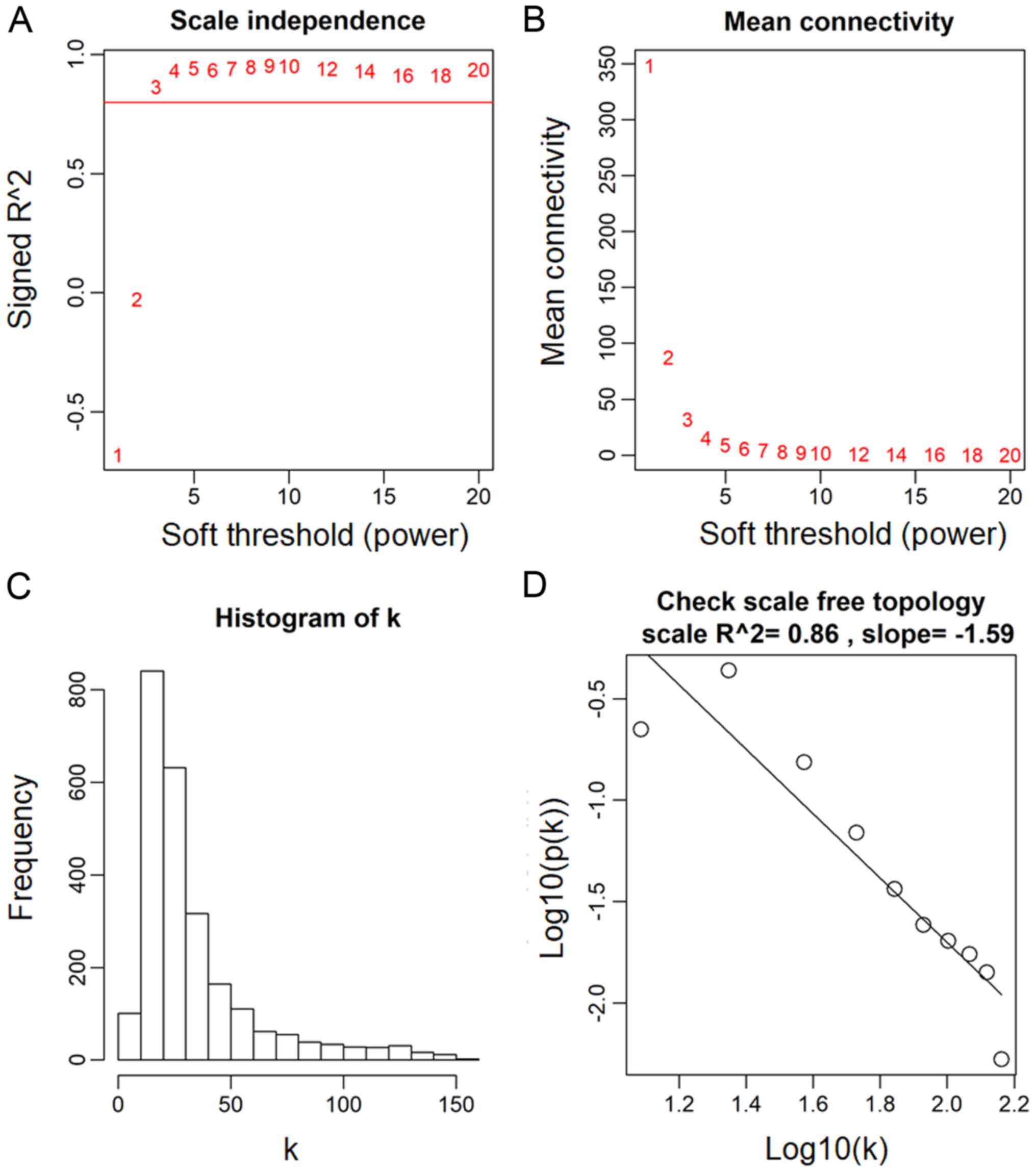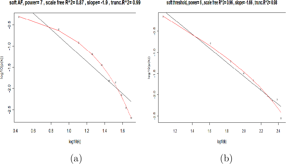Scale Free Topology refers to the frequency distribution of the connectivity k	The idea of check Scale Free Topology is to log transform p(k) and k and look at scatter plots.
With different beta, the linear model fitting R^2 index can show different goodness of fit and thus help us to select an appropriate beta value. In practive we use the lowest value where the curve starts to "saturate". And as beta increases, the mean connectivity decreases.	...

The scale free topology criterion for choosing the parameter values of an adjacency function

Consider only those parameter values in the adjacency function that result in approximate scale free topology, i.e, high scale free topology fitting index $R^2$

Rationale:

• Empirical finding: Many co-expression networks based on expression data from a single tissue exhibit scale free topology
• Many other network e.g. protein-protein interaction networks have been found to exhibit scale free topology

Caveat: When the data contains few very large modules, then the criterion may not apply. In this case, use the default choices.

Measure interconnectedness in a network

• adjacency matrix
• topological overlap matrix

Topological overlap matrix and corresponding dissimilarity

• TOM: short for Topological Overlap Matrix
• $\text{TOM}{ij} = \cfrac{\sum{u} a_{iu} a_{uj} + a_{ij} }{\min(k_{i},k_{j}) + 1 - a_{ij}}$
• $\text{DistTOM}{ij} = 1 - \text{TOM}{ij}$
• Generalization to weighted networks is straightforward since the formula is mathematically meaningful even if the adjacencies are real numbers in [0,1]
• Generalized topological overlap (Yip et al (2007) BMC Bioinformatics)
  • $\text{TOM}(i,j)=\cfrac{\lvert N_1(i)\cup N_1(j)\rvert+a_{ij}}{\min(\lvert N_1(i)\rvert, \lvert N_1(j)\rvert)+1-a_{ij}}$ for unweighted network

Noted that:

• $\sum_{u}a_{iu}a_{uj}\le\min(k_i,k_j)-a_{ij}$
• $\lvert N_1(i)\cup N_1(j)\rvert\le\min(\lvert N_1(i)\rvert, \lvert N_1(j)\rvert)-a_{ij}$
• $N_1(i)$ denotes the set of 1-step neighbors of node i
• $\lvert\rvert$ measures the cardinality
• Adding 1 to the denominator prevents it from becoming 0
• Therefore, $0\le a_{ij}\le1$ implies $0\le\text{TOM}_{ij}\le1$

Detect Network Modules(Clusters)

Module Definition

• We often use average linkage hierarchical clustering coupled with the topological overlap dissimilarity measure
• Based on the resulting cluster tree, we define modules as branches
• Modules are either labeled by integers (1,2,3…) or equivalently by colors

Two types of branch cutting methods

• Constant height (static) cut
  • simple, but requires careful choice of height and not suitable for complicated dendrograms with nested clusters
• Adaptive (dynamic) cut
  • Two version: Tree and Hybrid
  • Both look at the shape of the branches on the dendrogram, height and size information. Small clusters can be merged with neighboring large clusters
  • Hybrid conbines dendrogram cutting and PAM and retains advantages of both
    • no need to specify number of cluster
    • roustness (deal with background noise)

Visualize Network

• Topological overlap matrix plot (aka. connectivity plot)
• Multidimensional scaling (MDS)
• Heatmaps of modules
• external sortware (Traditional View):
  • ViSANT
  • Cytoscape
  • …

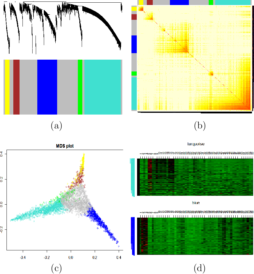Topological Overlap Plot: Modules correspond to branches of the dendrogram. Since modules are sets of nodes with high topological overlap, modules correspond to red squares along the diagonal. As in all hierarchical clustering analyses, it is a judgement call where to cut the tree branches.

Multidimensional Scaling: Use network distance in MDS

Heatmap View of Module: Since the genes of a module (rows) are highly correlated across microarray samples (columns), one observes vertical bands. The expression profiles are standardized across arrays. Red corresponds to high- and green to low expression values.

Summarize the expression profiles in a module

• Math Answer: Module eigengene = first principal component
• Network Answer: the most highly connected intramodular hub gene
• Both turn out to be equivalent

Module eigengene

Module eigen-gene = measure of over-expression = average redness

Using the singular value decomposition to define (module) eigengenes:

• Scale the gene expression profiles (columns)
• $\text{datX}=\text{scale}(\text{datX})$
• $\text{datX}=UDV^T$
• $U=(u_1, u_2, \ldots, u_m)$
• $V=(v_1,v_2, \dots,v_m)$
• $D=\text{diag}(\lvert d_1\rvert,\lvert d_2\rvert,\ldots,\lvert d_m\rvert)$
• …

Usefulness

• They allow one to relate modules to each other
  • Allow one to determine whether modules should be merged
  • Or to define eigengene networks
• They allow one the relate modules to clinical traits and SNPs
  • avoids multiple comparision problem
• They allow one to define a measure of module membership: $\text{kME}=\text{cor}(x,\text{ME})$
  • kME: Module Eigengene based Connectivity
  • ME: Module Eigengene

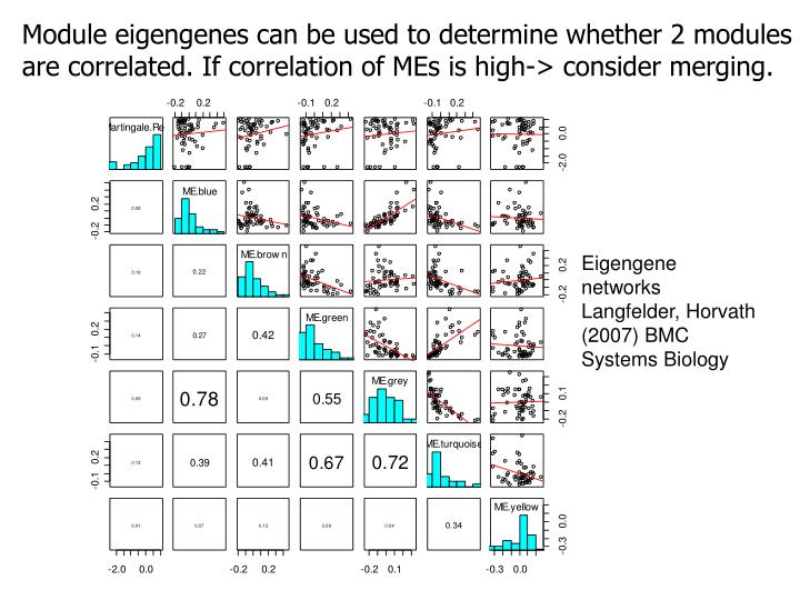Module eigengenes can be used to determine whether 2 modules are correlated. If correlation if MEs is high -> consider merging

Module detection in very large data sets

1. Variant of k-means to cluster variables into blocks
2. Hierarchical clustering and branch cutting in each block
3. Merge modules across blocks (based on correlations between module eigengenes)

Relate Modules to External Data

Clinical trait (e.g case-control status) give rise to a gene significance measure

• Abstract definition of a gene significance measure
  • GS(i) is non-negative
  • the bigger, the more “biological” significant for the i-th gene

Equivalent definition:

• $\text{GS.ClinicalTrait}(i)=\lvert \text{cor}(x(i),\text{ClinicalTrait})\rvert$ where x(i) is the gene expression profile of the i-th gene
• $\text{GS}(i)=\lvert \text{T-test}(i)\rvert$ of differetial expression between groups defined by the trait
• $\text{GS}(i)=-\log(\text{p-value})$

A gene significance naturally gives rise to a module significance measure:

• Define module significance as mean gene significance
• Often highly related to the correlation between module eigengene and trait

Important Task in Many Genomic Application: Given a network(pathway) of interactiong genes how to find the central players

• Connectivity can be an important variable for identifying important nodes
• Hub genes with respect to the whole network are often uninteresting (especially in coexpression networks)
  • but genes with high connectivity in interesting modules can be very interesting
• Define 2 alternative measures of intramodular connectivity for finding intramodular hubs
  • Intramodular connectivity $\text{kIN}$: Row sum across genes inside a given module: $\text{kIN}(i)=\sum_{j\in\text{ModuleSet}}a_{ij}$
    • Advantages: defined for any network based on adjacency matrix
    • Disadvantage: strong depends on module size
  • Module eigengene based connectivity $\text{kME}$ (also known as module membership measure): $\text{kME}=\text{ModuleMembership}(i)=\text{cor}(x_i,\text{ME})$
    • it is simply the correlation between i-th gene expression profile and the module eigengene
    • close to 1 means that the gene is a hub gene
    • Very useful measure for annotating gengs with regard to modules
    • Can be used to find genes that are members of two or more modules (fuzzy clustering)
    • Module eigengene can be interpreted as the most highly connected gene
• $\cfrac{\text{kIN}_{i}}{\max(\text{kIN})}\approx\lvert \text{cor}(x_i,E)\rvert^{\beta}=\lvert \text{kME}(i)\rvert^{\beta}$
  • $\lvert \text{kME}(i)\rvert^{\beta}$ measures group conform behavior

Intramodular hub genes

• Defined as genes with high kME (of high kIN)
• Single network analysis: Intramodular hubs in biologically interesting modules are often very interesting
• Differential network analysis: Genes that are intramodular hubs in one condiction but not in another are often very interesting

Reference

1. Zhang B, Horvath S. A general framework for weighted gene co-expression network analysis. Stat Appl Genet Mol Biol. 2005;4:Article17. doi:10.2202/1544-6115.1128
2. Langfelder, P., Horvath, S. Eigengene networks for studying the relationships between co-expression modules. BMC Syst Biol 1, 54 (2007). https://doi.org/10.1186/1752-0509-1-54
3. Horvath S, Dong J. Geometric interpretation of gene coexpression network analysis. PLoS Comput Biol. 2008;4(8):e1000117. Published 2008 Aug 15. doi:10.1371/journal.pcbi.1000117