Introduction to Gromacs

Steps to Run MD Simulation

1. Prepare Your System
   • Create Molecule: -avogadro
   • Create Topology: -topologn
   • gmx insert-molecules
   • gmx solvate
   • gmx grompp
   • gmx genion
2. Energy Minization
   • gmx grompp
   • gmx mdrun
   • gmx energy
3. Equilibration Run
   • gmx grompp
   • gmx mdrun
4. Production Run
   • gmx grompp
   • gmx mdrun
5. Analysis

The work-horse of the GROMACS package is the program mdrun. This program does not read the .top, .gro, or .mdp files directly, but requires a pre-processing step. This is done by the program grompp, which delivers a tpr-file (extension .tpr) if all goes well.

NOTE: before issuing the command mdrun, make sure the .tpr-file was created by grompp! If that step fails you will either not be able to run a simulation or you will repeat a simulation you had already done!

PREPARING THE SYSTEM

Missing residues, missing atoms and non-standard groups

The first step in the sequence then is the selection of a starting structure. The second step should be checking whether the structure has missing residues and atoms, which should be modeled in some way.

Another problem which one should be aware of is that structure files may contain non-standard residues, modified residues or ligands, for which force field parameters are not yet available. Such groups should either be removed or parameters should be determined for them, which is an advanced topic in MD.

Structure quality

It is good practice to run further checks on the structure to assess the quality. For instance, the refinement process in crystal structure determination may not always yield proper orientations of glutamine and asparagine amide groups. Also, the protonation state and side chain orientation of histidine residues may be problematic. To perform a proper validation of the structure, several programs and servers exist (e.g. WHATIF).

STRUCTURE CONVERSION AND TOPOLOGY

A molecule is defined by the coordinates of the atoms as well as by a description of the bonded and nonbonded interactions.

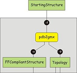
Since the structure obtained from the PDB only contains coordinates, we first have to construct the topology, which describes the system in terms of atom types, charges, bonds, etc. This topology is specific to a certain force field and the force field to be used is one of the issues requiring careful consideration. (e.g AMBER all-atom force field)

It is important that the topology matches with the structure, which means that the structure needs to be converted too, to adhere to the force field used. To convert the structure and construct the topology, the program pdb2gmx can be used. This program is designed to build topologies for molecules consisting of distinct building blocks, such as amino acids. It uses a library of building blocks for the conversion and will fail to recognize molecules or residues not present in the library. Issue the following command to convert the structure; choose the AMBER99SB force field and the TIP3P water model when prompted. Note the flag -ignh, which causes hydrogen atoms present in the file to be removed, and to be rebuild according to the description in the force field.

1

gmx pdb2gmx -f protein.pdb -o protein.gro -p protein.top -ignh

Read through the output on the screen and check the choices made for the histidine protonation and the resulting total charge of the protein. Also browse through the input structure file (protein.pdb, pdb format) and output structure file (protein.gro, gromacs format). Note the differences between the two formats. Also note that the output structure file could as well have been chosen to be in pdb format. Now browse through the topology file (open the file protein.top in an editor, such as gedit) and look at the structure of the topology file and the information specified in it.

Note:

• Write down the number of atoms before and after the conversion and explain the difference if any
• List the index numbers, atoms, atom types and charges from the tryptophan residue as given in the topology file

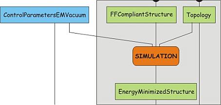
ENERGY MINIMIZATION OF THE STRUCTURE (VACUUM)

Now a structure is generated in the correct format for the force field chosen, as well as the corresponding topology. However, the conversion of the structure involves the deletion and or addition of hydrogen atoms and may cause strain to be introduced, e.g. due to atoms positioned too close together. Therefore, we have to perform an energy minimization on the structure, and let it relax a bit. This is in fact a simulation step, and involves two processes. First, the structure and the topology are combined into a single description of the system, together with a number of control parameters. This yields a run input file, which can be used as the single input for the simulation program mdrun. The advantage of splitting the two sub-processes is that the run-input file can be transferred to a dedicated (high-performance) computer network or a supercomputer and be processed there. However, this is only relevant for the production simulation.

To perform these steps first save the parameter file minim.mdp to your directory. You can do this, by right-clicking on the link and choosing your working directory as the download site, or download to your Download folder and copy it from there. The file should be in the directory where you want to do the simulation, otherwise you will get an error ‘file not found’. This file contains the control parameters for the energy minimization. Have a look at the contents of this file. Notice the line starting with “integrator”, which specifies the algorithm to be used. In this case it is set to perform a steepest descent energy minimization of 500 steps. Now, combine the structure, topology and control parameters using grompp:

1

gmx grompp -f minim.mdp -c protein.gro -p protein.top -o protein-EM-vacuum.tpr

grompp will note that the system has a non-zero charge and will print some other information regarding the system and the control parameters. The program will also generate an additional output file, which contains the settings for all control parameters (mdout.mdp).

make sure the file protein-EM-vacuum.tpr was created by grompp!

Now, continue with mdrun:

1

gmx mdrun -v -deffnm protein-EM-vacuum -c protein-EM-vacuum.pdb -nt 1

Since there are only few atoms, the energy minimization finishes quickly. The -v flag causes the potential energy and the maximum force to be printed at each step, which allows you to follow how the minimization is progressing. The option -nt 1 causes the program to use only 1 CPU, which is actually better for such a small molecule. Later on, we will use the multiple CPUs.

The structures before and after energy minimization by loading them into PyMol (first convert the starting structure from .gro to .pdb format; enter the number for the group “System” when prompted):

1

gmx trjconv -s protein-EM-vacuum.tpr -f protein.gro -o protein-from-PDB.pdb

1

pymol protein-from-PDB.pdb protein-EM-vacuum.pdb

Alternatively, use VMD (visual molecular dynamics):

1

vmd protein-from-PDB.pdb protein-EM-vacuum.pdb

It is interesting to have a look at what happens with the potential energy. The energy information from the simulation is stored in an unreadable (binary) file format with extension .edr. The information in this file can be extracted using the gromacs tool gmx energy. Next, the extracted information can shown as a plot or a graph. Start extracting the potential energy:

1

gmx energy -f protein-EM-vacuum.edr -o potential-energy-EM.xvg

This will present you a list of energy terms you can select for writing to the file given for output. Find the number that corresponds to the potential energy and enter it. Then type a 0 (zero) and press enter.

The output file (.xvg) can be viewed with the program ‘xmgr’ or ‘xmgrace’, one of which should be installed. On the LWP at the University of Groningen:

1

xmgrace potential-energy-EM.xvg

Note:

• Which method was used for the energy minimization?
• How many steps were specified in the parameter file and how many steps did the minimization take?
• What could cause the energy minimization to stop before the specified number of steps was reached?
• What is the final potential energy of the system?
• What happens to the potential energy?
• Is the information on the horizontal axis in the graph potential-energy-EM.xvg correct?

Now that the structure is relaxed, it is time to set up the periodic boundary conditions and add the solvent.

PERIODIC BOUNDARY CONDITIONS

Before adding the solvent, a general layout (the space) of the simulation setup has to be chosen. Most commonly simulations are performed under periodic boundary conditions (PBC), meaning that a single unit cell is defined, which can be stacked in a space filling way. In this way, an infinite, periodic system can be simulated, avoiding edge effects due to the walls of the simulation volume. There are only a few general shapes available to set up PBC. We will use a rhombic dodecahedron because it corresponds to the optimal packing of a sphere, and is therefore the best choice for freely rotating molecules. To disallow direct interactions between periodic images we set a minimal distance of 1.0 nm between the protein and the wall of the cell, such that no two neighbours will be closer than 2.0 nm. Periodic boundary conditions are set with editconf:

1

gmx editconf -f protein-EM-vacuum.pdb -o protein-PBC.gro -bt dodecahedron -d 1.0

Have a look at the output of editconf, and note the changes in the volume.

NOTE:

What is the new unit cell volume?

Also, have a look at the last line of the file protein-PBC.gro:

1

tail -1 protein-PBC.gro

In the gromacs format (.gro), the last line specifies the unit cell shape. It always uses the triclinic matrix representation, with the first three numbers specifying the diagonal elements (xx, yy, zz) and the last six giving the off-diagonal elements (xy, xz, yx, yz, zx, zy).

SOLVENT ADDITION

Now that the unit cell is set up, solvent can be added. There are several solvent models, each of which is more or less intimately linked to a force field. The GROMOS force fields are generally used with the simple point charge (SPC) water model. The topology is not required for solvent generation, but may be updated to include the solvent added. To fill the unit cell with SPC issue the following command:

1

gmx solvate -cp protein-PBC.gro -cs spc216.gro -p protein.top -o protein-water.pdb

Have a look at the end of the file protein.top to see the addition, and check the numbers with the amount of solvent added according to genbox.

NOTE:

• How many water molecules are added to the system?
• How many atoms are in the system now?

Load the solvated structure (protein-water.pdb) in Pymol. In Pymol, the unit cell can be visualized using the command

1

show cell

With VMD, type the following in the terminal from which you started vmd:

1

pbc box

This draws a wireframe, showing the edges of the triclinic unit cell. Although it may not be obvious, this triclinic shape corresponds to a rhombic dodecahedron. Another thing to note is that the solvent is not all inside the unit cell, but is arranged as a rectangular brick. Quite likely, the protein is partially sticking out of the water.

NOTE:

• Why is it not a problem to have the protein sticking out of the water?

ADDITION OF IONS: COUNTER CHARGE AND CONCENTRATION

At this point, we have a solvated protein, but the net charge of the system still remains. To make the system neutral we have to add a number of counterions. In addition, it may be considered good practice to add ions up to a certain concentration. The program genion can take care of both tasks, but requires a run input file as input, i.e. a file containing both the structure and the topology. As we saw before, such a file can be generated with grompp:

1

gmx grompp -v -f minim.mdp -c protein-water.pdb -p protein.top -o protein-water.tpr

Subsequently, the file protein-water.tpr can be used as input for genion. We specify a concentration of 0.15 M (-conc 0.15) of NA+/CL- (-pname NA -nname CL) to be added and indicate that an excess of one species of ion has to be added to neutralize the system (-neutral). genion will ask for a group of molecules to be used to partly replace with ions. The group ‘SOL’ should be chosen. Type the number from the list corresponding to this group and press ‘Enter’. Before you do this, make a copy of the topology file without the ions:

1
2
3

cp protein.top protein-water.top

gmx genion -s protein-water.tpr -o protein-solvated.gro -conc 0.15 -neutral -pname NA -nname CL -p protein.top

Note the numbers of ions added, and verify that an excess of negative or positive ions is added for neutralization. Having replaced a number of water molecules with ions, the system topology in protein.top has changed! Compare the last lines of the files protein-water.top and protein.top and check that the differences reflect what has just been done by the genion program.

Recently the naming of ions in Gromacs changed. For Gromacs versions 4.5.3 and higher it may be necessary to use the ion names NA/CL rather than NA+/CL-. In that case, you need to edit the file protein.top yourself.

1

gedit protein.top

NOTE:

• How many sodium and chloride ions are added to the system?

At this stage, we should have a starting structure of the peptide in solvent (water) and ions to the peptide and gently get the system ready for a production simulation. In view of the available time, a script implements the next steps so you do not have to do all the typing. Save this script under the name ‘SETUP-SOLVATED-PEPTIDE’. Please set the script to work and in the meantime read on to understand what steps are being taken to generate a system of a peptide in solvent and containing ions. If you have some time left, you can study this part in more detail, performing the analysis steps as well.

1
2
3

chmod 755 SETUP-SOLVATED-PEPTIDE

./SETUP-SOLVATED-PEPTIDE

After the script is finished CORRECTLY, we can skip some of the steps below (because they are taken care of by the script just run) and we resume the tutorial at the point where a (short) production run can be started here. In case you got errors, try to solve them by finding out where it all went wrong or call your tutorial assistant for trouble shooting!

ENERGY MINIMIZATION OF THE SOLVATED SYSTEM

Now the whole simulation system is defined. The only steps before starting a production run involve the controlled relaxation of the system. The generation of solvent as well as the placement of ions, may have caused unfavourable interactions, e.g. overlapping atoms, equal charges too close together. Therefore, the system is energy minimized again, following the same steps as before, but now with periodic boundary conditions. Edit the file minim.mdp and change the line pbc = no to pbc = xyz Nerd solution!: sed -i /^pbc/s/no/xyz/minim.mdp. Then run grompp and mdrun:

1
2
3

gmx grompp -v -f minim.mdp -c protein-solvated.gro -p protein.top -o protein-EM-solvated.tpr

gmx mdrun -v -deffnm protein-EM-solvated -c protein-EM-solvated.gro

NOTE:

• How many steps were specified in the parameter file and how many steps did the minimization take?
• What is the final potential energy of the system?

RELAXATION OF SOLVENT AND HYDROGEN ATOM POSITIONS: POSITION RESTRAINED MD

With the greatest strain dissipated from the system, we now let the solvent adapt to the protein, i.e. we allow the solvent to move freely, while keeping the non-hydrogen atoms of the proteins more or less fixed to the reference positions. This is done to assure that the solvent configuration ‘matches’ the protein. This step is the first actual MD step. The control parameters for this step can be found in pr.mdp, which should be downloaded. Have a look at this file and note the integrator used as well as the define statement. The latter is used to allow flow control in the topology file. define = -DPOSRES will cause the keyword “POSRES” to be globally defined. Have a look at the end of the topology file to see how this is used to turn on position restraints. Use grompp and mdrun to run the simulation:

1
2
3

gmx grompp -v -f pr.mdp -c protein-EM-solvated.gro -p protein.top -o protein-PR.tpr

gmx mdrun -v -deffnm protein-PR

NOTE:

• What is the length of the simulation in picoseconds?
• How is the inclusion of the position restraints handled in the topology file?

It is interesting to have a look at what happens with the total, potential and kinetic energies. In the previous steps, the particles did not have velocity, so there was no kinetic energy and hence no temperature. Now, at the start of the simulation, the atoms were assigned velocities and with that got kinetic energy. Extract information about temperature, potential energy, kinetic energy, and total energy:

1
2
3
4
5
6
7

gmx energy -f protein-PR.edr -o temperature-PR.xvg

gmx energy -f protein-PR.edr -o potential-energy-PR.xvg

gmx energy -f protein-PR.edr -o kinetic-energy-PR.xvg

gmx energy -f protein-PR.edr -o total-energy-PR.xvg

View the graphs with xmgrace:

1

xmgrace temperature-PR.xvg

NOTE:

• What happens with the temperature?
• What happens to the potential/kinetic/total energy and how can this be explained?

UNRESTRAINED MD SIMULATION, TURNING ON TEMPERATURE COUPLING

The system should now be relatively free of strain. Time to turn up the heat, and start to couple the system to the heat bath. In other words, a short run will be performed in which the temperature coupling is turned on and the system is allowed to relax to the new conditions. Download the control parameter file nvt.mdp and have a look at the temperature coupling parameters in it. Then run the simulation, using grompp and mdrun:

1
2
3

gmx grompp -v -f nvt.mdp -c protein-PR.gro -p protein.top -o protein-NVT.tpr

gmx mdrun -v -deffnm protein-NVT

NOTE:

• There are two groups which are separately coupled to a heat bath. Which groups are that and what do you think is in each of these groups?

After the run finishes have a look at the energies and temperature. Extract them in the same way as before. Note again that you may want to start the next simulation before looking at the energies from this one.

1
2
3
4
5
6
7

gmx energy -f protein-NVT.edr -o temperature-NVT.xvg

gmx energy -f protein-NVT.edr -o potential-energy-NVT.xvg

gmx energy -f protein-NVT.edr -o kinetic-energy-NVT.xvg

gmx energy -f protein-NVT.edr -o total-energy-NVT.xvg

Have a look at the energy graphs.

NOTE:

• What happens to the temperature?
• What happens to the potential/kinetic/total energy and how can this be explained?

UNRESTRAINED MD SIMULATION, TURNING ON PRESSURE COUPLING

After relaxation of the temperature and the temperature coupling, it is time to start putting things under pressure. Perform a short simulation with pressure coupling turned on, using the control parameter file npt.mdp. Have a look at this file and identify the parameters controlling the pressure coupling.

Also note that we reassign velocities to the particles, which is controlled with the parameter gen_vel. Below that line, the temperature for the distribution of velocities (the Maxwell distribution) is set and the seed for the random number generator is specified (gen_seed). gen_seed is currently set to 9999, but should be changed to your group number. (Nerd solution: sed -i /^gen_seed/s/9999/YOURGROUPNUMBER/ npt.mdp) MD simulations are deterministic, so starting with the same set of coordinates and velocities and the same parameters would cause the outcomes of the simulations to be identical, which is not what we want.

After you’ve edited the parameter file, prepare and run the simulation:

1
2
3

gmx grompp -v -f npt.mdp -c protein-NVT.gro -p protein.top -o protein-NPT.tpr

gmx mdrun -deffnm protein-NPT

After the run finishes, again have a look at the energies, the temperature and the pressure. Extract them in the same way as before.

1
2
3
4
5
6
7

gmx energy -f protein-NPT.edr -o temperature-NPT.xvg

gmx energy -f protein-NPT.edr -o pressure-NPT.xvg

gmx energy -f protein-NPT.edr -o potential-energy-NPT.xvg

gmx energy -f protein-NPT.edr -o kinetic-energy-NPT.xvg

Have a look at the energy graphs, the temperature and the pressure.

NOTE:

• What happens to the temperature?
• What happens to the pressure?

The last question relates directly to the extraction of thermodynamic properties from systems consisting of limited numbers of particles. Thermodynamics is, crudely spoken, about the behaviour of large collections of particles; billions rather than thousands. Averaging a properties over many many particles will yield values which have small fluctuations. On the other hand, averaging over a small number of particles inevitably gives large fluctuation.

Since we now do pressure coupling, the density of the system may also change. Extract the density from the energy file too:

1

gmx energy -f protein-NPT.edr -o density-NPT.xvg

NOTE:

• How does the density behave over time?
• Why does the density of the system change if pressure coupling is turned on?

PRODUCTION SIMULATION

Now finally, we have a more or less equilibrated solvated system containing our peptide of interest and it is time to start a production simulation. Mind that production simulation does not imply that the whole simulation can be used for analysis of the properties of interest. Although some of the memory of the initial configuration has been erased, it is unlikely that the system has already reached equilibrium. In the analysis section we will investigate which part of the simulation can be considered in equilibrium and is thus suited for further processing. But first it is time to set up the simulation. This merely involves running another simulation step, similar to the last step of the preparation. However, this is another of these times where it is necessary to think about the purpose of the simulation. The control parameters have to be chosen such that the simulation will allow analysing the properties one has in mind. Questions to be addressed are:

• At what time scale do the processes of interest manifest themselves or how long should the simulation be run?
• How many frames are necessary, or what time resolution is required?
• Is there need to store velocities?
• Should all atoms be in the output, or is it sufficient to save only protein coordinates?
• What frequency should be used for writing energies and log entries?
• What frequency should be used for writing check point coordinates and velocities?
• …

NOTE: the simulation started below may be compared to other simulations started from the same structure, but under different conditions. In this tutorial, we will apply distance restraints to selected atom pairs. This is explained in a separate section, click here to enter that section.

We’re going to run a 2.0 nanosecond (2000 ps) simulation. The simulations will be run locally.

Download or copy the control parameter file md.mdp and have a look at the contents of it. You’ll have to edit the file and specify how many steps should be taken to get a total simulation time of 2000 ps. Then take the final structure file and topology resulting from the preparation and combine them into a run input file using grompp.

1
2
3
4
5

gedit md.mdp

gmx grompp -f md.mdp -c protein-NPT.gro -p protein.top -o topol.tpr

gmx mdrun >& md.job &

While your simulation is running, you can review the set-up process and then proceed to already do some of the analysis. The analysis programs will work on the part of the simulation that is already done, while the simulation is still running and producing more data.

Files in Gromacs

• System Topology topol.top
  • The definition of the molecule and the system (how many molecules of what type are present) reside in a file with an extension .top
• Molecule Topology topinc.itp
  • To enhance readability, the .top file may refer to other files containing information, with extension .itp, usually these contain the specification of the interactions (i.e. the force field)
• Molecule Coordinates conf.gro
  • Apart from information about the molecules and their interactions, a run requires starting coordinates. These may be provided in different formats, e.g. the PDB-format as downloaded from the database, or other. We will use the PDB and internal GROMACS formats most of the time. The extension of the internal GROMACS file-name is .gro
• Parameter File grompp.mdp
  • Finally, the run needs to know how many MD steps must be taken, what the temperature and pressure should be etc. All such information (“run-time variables”) are specified in a so-called mdp-file, extension .mdp

Geometry Files *.gro

Topology Files *.top and *.itp

Input File with MD Parameters *.mdp

Reference

1. http://cgmartini.nl/~mdcourse/pepmd/md.html
2. https://www.youtube.com/watch?v=KEfMuHMTBQU
3. https://www.youtube.com/watch?v=rYZ1p5lXNyc